Jason Becker
January 24, 2012

Ted Nesi has done a pretty solid job tracing the history of some awful decisions made by union-dominated boards that resulted in a significant number of retirees in the early-90s receiving 5% or 6% annually compounded interest on their retirement income. These are often called COLAs, or cost-of-living adjustments.

Today, I am inspired by Nesi’s post on the rapid decline of the Providence municipal pension fund health that occurred since 6% “COLA” was introduced in 1989 through today. You see, something has really been bugging me about the conversation on municipal pensions in Rhode Island. A true COLA is key to ensuring that purchasing power is maintained throughout retirement. Essentially, quality of life and ability to buy required goods should be consistent from the day you retire until the day you die. This is a goal that makes a lot of sense. But the cost of goods has not increased 5% or 6% year-over-year ever in the past twenty years 1.

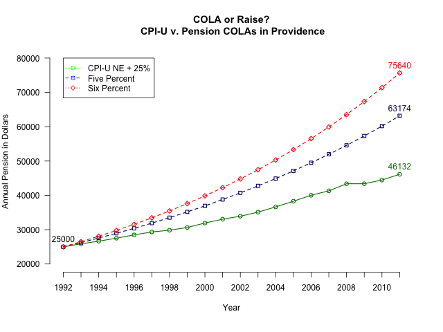
So I chose a key moment in the history of Providence municipal pensions– a 1991 consent decree 2 that then Mayor Buddy Cianci signed, solidifying and legitimizing the extremely high “COLA” for workers. I wanted to know, “What would a worker retiring in the following year (1992) be making today if they retired with a $25,000 annual pension and had a 6% ‘COLA’, 5% ‘COLA’, or a COLA based on the Northeast CPI-U?” Not wanting to make a key mistake and equate a CPI with a COLA, I increased the CPI-U for each year by 25%, figuring that this is a reasonable approximation of the marginal taxes that would be paid on additional income by these retirees.

I suspected that 5% and 6% do not really result in a cost-of-living adjustment, but rather a clear wage increase for retired workers. I have no problem maintaining parity or near-parity with retirement level income, but there’s absolute no reason someone who retired should receive a wage. My support for a true COLA is so strong that I made the adjustment for taxes on income!

What were the results?
Inflation1

A Providence employee who retired in 1992 with a $25,000 pension would be receiving $46,132 in 2011 if their retirement was increased by inflation + the marginal tax rate (assumed here as 25%). But a Providence employee who retired with the same pension in 1992 under the conditions in Providence could expect $63,174 at 5% or $75,640 at the 5% and 6% rates, respectively. This is a MASSIVE difference which cannot constitute a “COLA”.

So I move that we stop referring to these particular pensions as having a “COLA”, because what really happened was a fixed raise was created to last for the rest of retirees’ lives.

Some additional neat facts:

Over 20 years, an individual who has a 6% raise per year will have collected $228,672 more than someone who had a COLA. An individual with a 5% raise per year will have collected $135,681.10 over the same 20 year period.

And of course, here’s the code I used to produce the graph above in R3:

 1
 2
 3
 4
 5
 6
 7
 8
 9
10
11
12
13
14
15
16
17
18
19
20
21
22
23
24
25
26
27
28
29
30
31
32
33
34
35
36
37
38
39
40
41
42
43
44
45
46
47
48
49
50
51
52
53
compound <- function(start,rate,timespan){
  x <- vector(mode = 'numeric', length = timespan)
  for(i in 1:timespan){
    if(i == 1){
      x[i] <- start
    }
    else{
          x[i] <- x[i-1]*(1+rate)
    }
  }
  return(x)
 }
    
inflate <- function(start, inflation){
  x <- vector(mode='numeric', length=dim(inflation)[1])
  for(i in 1:dim(inflation)[1]){
    if(i==1){
      x[i] <- start
    }
    else{
      x[i] <- x[i-1]*(1+(1.25*(inflation[i,2]/100)))
    }
  }
  return(x)
}

cpiu <- cbind(seq(from=1992,to=2011), c(0.0, 2.8, 2.4, 2.6, 2.8, 2.4, 1.4, 
                                        2.1, 3.4, 2.8, 2.1, 2.8, 3.5, 3.6,
                                        3.6, 2.6, 4.0, 0.0, 2.0, 3.0))

inflation <- data.frame(cbind(cpiu[,1], inflate(25000, cpiu), 
                              compound(25000, .05, 2), 
                              compound(25000, .06, 20)))

names(inflation) <- c('year', 'NECPI.U', 'FivePercent', 'SixPercent')
png(filename="inflation.png", height=640, width=800, bg="white")
par(mar=c(6, 5, 5, 3))
plot(inflation$NECPI.U, type='o', col=rgb(0,0.5,0), ylim=c(20000,80000), 
     axes=FALSE, ann=FALSE, lwd=1.5)
axis(1, at=1:20, lab=inflation$year)
axis(2, las=1, at=seq(from=20000, to=80000, by=10000))
lines(inflation$FivePercent, type="o", pch=22, lty=2, col=rgb(0,0,0.5), 
      lwd=1.5)
lines(inflation$SixPercent, type="o", pch=23, lty=2, col='red', lwd=1.5)
title(main="COLA or Raise?\n CPI-U v. Pension COLAs in Providence", col.    main="black")
title(xlab="Year")
title(ylab="Annual Pension in Dollars\n")
legend(1, 80000, c('CPI-U NE + 25%', 'Five Percent', 'Six Percent'), col=c(   'green', 'blue', 'red'), pch=21:23, lty=1:3)
text(1,25000, 25000, pos=3, col='black')
text(20, max(inflation$SixPercent), round(max(inflation$SixPercent), 0), pos=3,     col='red')
text(20, max(inflation$FivePercent), round(max(inflation$FivePercent), 0)   ,pos=3, col=rgb(0,0,0.5))
text(20, max(inflation$NECPI.U), round(max(inflation$NECPI.U), 0), pos=3,     col=rgb(0,0.5,0))
dev.off()

This post reflects my personal views and opinions. I am a member of Local 2012 of the RIAFT and was a supporter of the statewide pension reform in the Fall of 2011. I am also a resident of Providence.


  1. Consumer Price Index Northeast from the Bureau of Labor Statistics ↩︎

  2. See the first link in this post ↩︎

  3. Sorry this code is not well-commented, but I believe it’s fairly straight forward ↩︎
January 22, 2012

The past few months I’ve been learning how to use R. This morning, I decided to try out two first– importing a table of data that is being read of the web and overlaying location data onto a map.

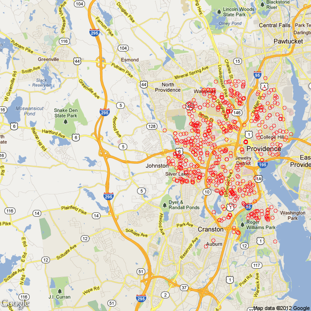
With a little bit of Google skills and just enough R know-how I was able to produce this image:

Homesales

There were a few things that were kind of tricky for me. First, for sometime I couldn’t get latitude and longitude components for the addresses. I figured there was something wrong with the way I was using the *apply class of functions in R. apply() (and the related class of functions lapply, sapply, etc.) are really handy if a bit tricky for beginning R users. This function permits quickly “applying” a function across multiple elements. Traditionally this is done with a loop, but the apply() functions “vectorize” this process (R folks always talk about making your code more vectorized which has something to do with the structure of objects in R but is beyond my computer science skills– essentially, vectorized code runs much faster and more efficiency than loops because of some underlying feature of the language). After playing around with apply, lapply, and sapply, I decided to move back into my “old” way of thinking and just write a loop:

 1
 2
 3
 4
 5
 6
 7
 8
 9
10
latlongroll <- function(address){
  lat <- vector(mode = "numeric", length = length(address))
  lng <- vector(mode = "numeric", length = length(address))
  for(i in 1:length(address)){
    latlong <- gGeoCode(address[i])
    lat[i]<-latlong[1]
    lng[i]<-latlong[2]
  }
  return(cbind(lat,lng))
} 

This still didn’t work– I kept on getting a strange out-of-bounds call. So I decided to go down the rabbit hole of regular expressions and try and see if I could clean up my addresses any further (I couldn’t). So, now seemed as good a time as any to figure out how to print to the console while a loop is running to keep track of progress and where exactly my function was stopped. This turned out to be a bit tricky because I didn’t know you had to include a tricky line, r flush.console() in order to get the prints to work. When I figured this out I found out my loop was being caught on my 7th element, a perfectly well formed address. When I ran gGeoCode() on that address only it worked fine. So I thought, maybe Google is bouncing me out because I’m hitting it too fast? And bingo, the final (working version):

 1
 2
 3
 4
 5
 6
 7
 8
 9
10
11
12
13
latlongroll <- function(address){
 lat <- vector(mode = "numeric", length = length(address))
 lng <- vector(mode = "numeric", length = length(address))
 for(i in 1:length(address)){
  print(i)
  flush.console()
  latlong <- gGeoCode(address[i])
  lat[i]<-latlong[1]
  lng[i]<-latlong[2]
  Sys.sleep(0.5)
 }
 return(cbind(lat,lng))
}

Other than that, the whole process was pretty straight forward. I have to thank Tony Breyal for posting the functions I used to get latitude and longitude on Stack Overflow. Also, I found the RgoogleMaps vignette to be very helpful, although I wish it had slightly better explained what was going on in qbbox().

Finally, my full source for the above:

 1
 2
 3
 4
 5
 6
 7
 8
 9
10
11
12
13
14
15
16
17
18
19
20
21
22
23
24
25
26
27
28
29
30
31
32
33
34
35
36
37
38
39
40
41
42
43
44
45
46
47
48
49
50
51
52
53
54
55
56
57
58
59
60
61
62
63
64
65
66
67
68
69
70
71
72
# Providence Real Estate Transactions over the last 40 days.
# Required Packages
require('XML')
require('RCurl')
require('RJSONIO')
require("RgoogleMaps")
# Functions
# Construct URL required to get the Lat and Long from Google Maps
construct.geocode.url <- function(address, return.call = "json", sensor = "false"   ) {
 root <- "[maps.google.com/maps/api/...](http://maps.google.com/maps/api/geocode/)"
 u <- paste(root, return.call, "?address=", address, "&sensor=", sensor, sep = ""   )
 return(URLencode(u))
}
# Now that we have the proper Google Maps address, get the resulting latitude     and longitude
gGeoCode <- function(address) {
 u <- construct.geocode.url(address)
 doc <- getURL(u)
 x <- fromJSON(doc,simplify = FALSE)
 lat <- x$results[[1]]$geometry$location$lat
 lng <- x$results[[1]]$geometry$location$lng
 return(c(lat, lng))
}
# Roll through addresses to create lat long
latlongroll <- function(address){
# Initializing the length of a vector dramatically speeds up the code. Far 
# better than reassigning and resizing each time in the loop.
 lat <- vector(mode = "numeric", length = length(address))
 lng <- vector(mode = "numeric", length = length(address))
 for(i in 1:length(address)){
# I kept the print in because this function takes a long time to run so I 
# like  to watch its progress.
 print(i)
 flush.console()
# To reduce the calls, I chose to store lat and long locally before 
# separating the two whereas initially I hit Google for each separately
 latlong <- gGeoCode(address[i])
 lat[i]<-latlong[1]
 lng[i]<-latlong[2]
# I'll have to experiment with the sleep time. I'm certain 0.5 seconds is 
# too long (and this is the bulk of the time spent on the whole code).
 Sys.sleep(0.5)
 }
 return(cbind(lat,lng))
}

# Open to the most recent real estate transactions for Providence on the 
# Projo
site <- '[www.providencejournal.com/homes/rea...](http://www.providencejournal.com/homes/real-estate-transactions/assets/pages/real-estate-transactions-providence.htm')
# Read in the table with the header as variable names.
realestate.table<-readHTMLTable(site,header=T,which=1,stringsAsFactors=F)
# Remove the $ sign before the price
realestate.table$Price <- gsub("([$]{1})([0-9]+)", "\\2", 
                               realestate.table$Price)
# Cast price character as numeric
realestate.table$Price<-as.numeric(realestate.table$Price)
# Cast date string as date type (lowercase %y means 2-digit year, 
# uppercase is 4 digit)
realestate.table$Date <- as.Date(realestate.table$Date,format='%m/%d/%y')
# Dummy transactions or title changes have a price of $1, removing those 
# from data set
providence <- subset(realestate.table,Price>1)
# Removing properties that do not have an address that start with a street 
# number
providence <- subset(providence, grepl("^[0-9]+", providence$Address))
# Add lat and lng coordinates to each address
providence<-cbind(providence, latlongroll(providence[,3]))
# Calculate boundary lat and long for map
bb <- qbbox(providence$lat, providence$lng)
# Gets a map from Google Maps
map <- GetMap.bbox(bb$lonR, bb$latR, zoom=12, maptype="mobile")
# plot the points
PlotOnStaticMap(map,lon=providence$lng,lat=providence$lat)
December 18, 2011

If you’re just beginning to use R and want a quick and easy way to make some charts/graphs, etc, GrapheR is a great package to quickly produce high quality plots through a self-explanatory GUI. Here’s an article in The R Journal today.

My only complaint is that GrapheR does not appear to have a way to export the code that produced the graph, which would be a very helpful feature for a beginner who wants to learn the guts of producing publication quality charts in R.

To install and then run…

1
2
3
install.packages('GrapheR')
require(GrapheR)
run.GrapheR()